Using Custom Telemetry Data in an IBA Probe
SUMMARY This topic describes how to create an IBA probe and detect and store any anomalies in a historical database for reference.
So far in our walkthrough, we've created a custom telemetry collector service that defines the data you want to collect from your devices. Now let's ingest this data into IBA probes in your blueprint so that Apstra can visualize and analyze the data.
Create a Probe
Data Center and Freeform blueprints support IBA probes with the Custom Telemetry Collection.
-
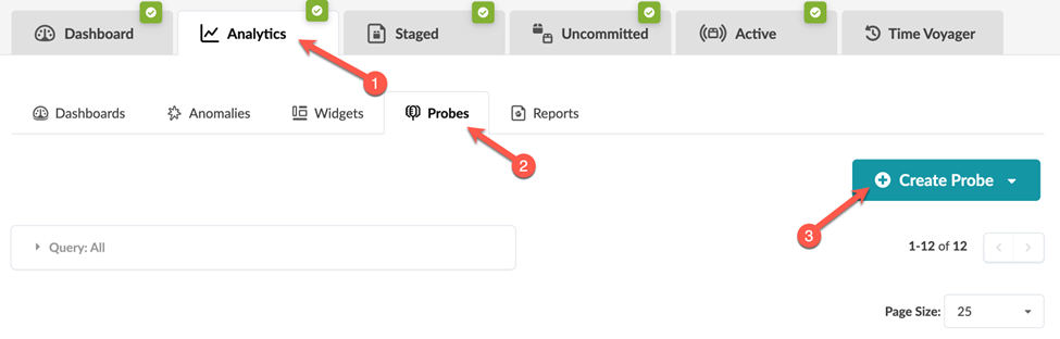
From your blueprint, navigate to Analytics >
Probes, and then click Create Probe > New
Probe.
-
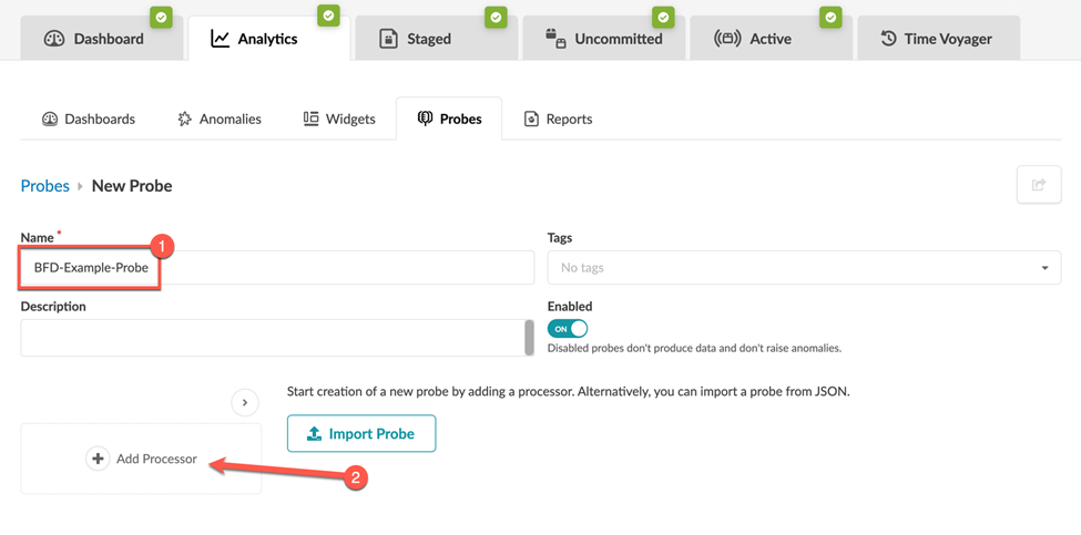
Enter a name and (optional) description (in this example,
BFD-Example-Probe), then click Add
Processor.
-
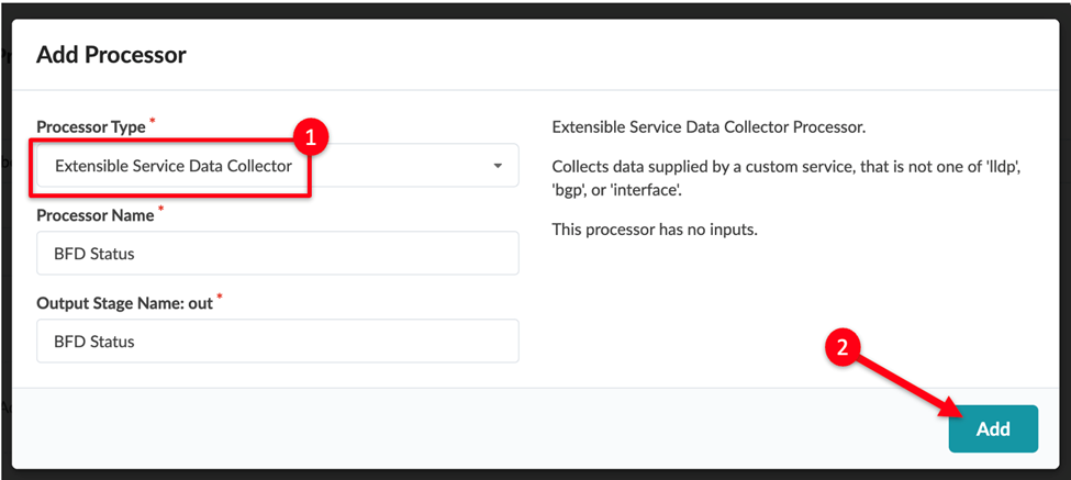
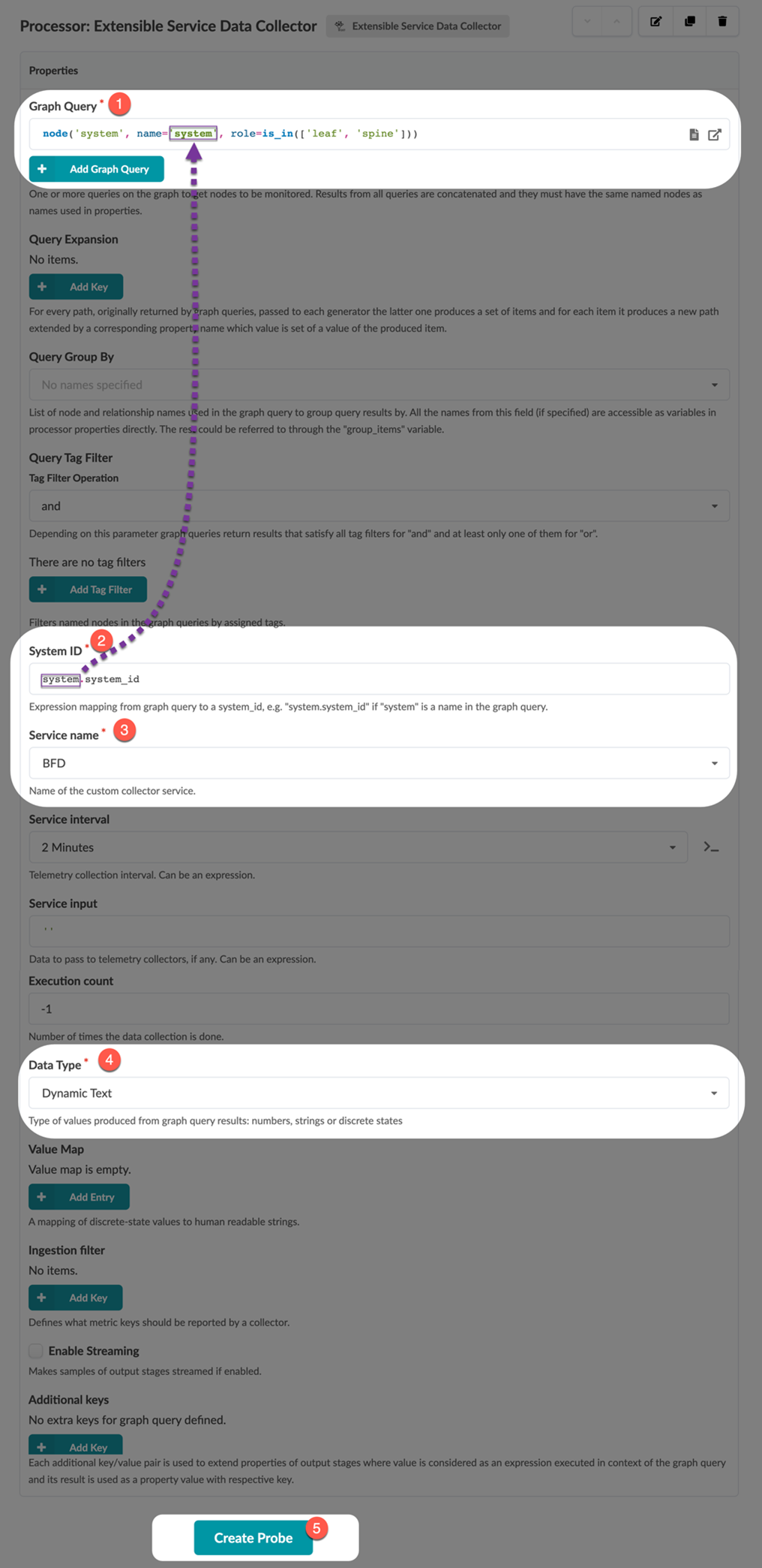
Select a processor type. For our example, we selected the
Extensible Service Data Collector
processor.
-
To the right of the Graph Query field click the Select a predefined
graph query button, then select DC – All managed devices (any
role) from the Predefined Query
drop-down.
This query determines the scope within the blueprint in which the telemetry collection is executed. This means if a device in your blueprint is not matched by the graph query, the telemetry collection service will not start for that device.
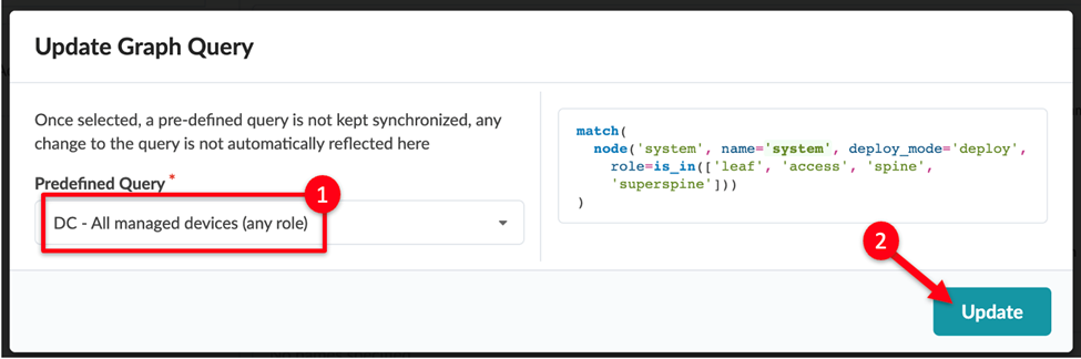
The graph query specifically matches all system nodes in the graph database of your blueprint. Each managed device, such as a leaf switch or spine switch, shows as a
systemnode in the graph.In the Predefined Query we selected above, the query matches all nodes of the type
system, which in deploy mode has a role ofleaf,access,spine, orsuperspine. -
Click Update to return to the table view.
-
Navigate to the output stage of the data collector processor to verify that
the probe is correctly ingesting data from your custom telemetry
collector.
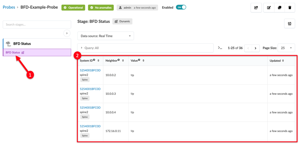 Congratulations! You successfully create a probe!
Customize a Probe
We created a working probe that collects the BFD state for every device in your network. Now let’s explore a couple of useful customization options to fine-tune your probe.
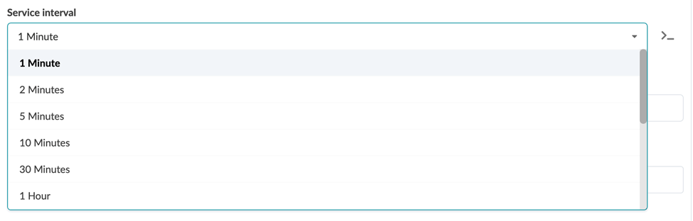
Service Interval
The service interval determines how often your telemetry collection service fetches data from devices and ingests them into the probe. This interval is an important parameter to be aware of because an overly aggressive interval can cause excessive load on your devices. The optimal interval will depend on the data you are collecting. For example, a collector fetching the content of a large routing table with thousands of entries can cause a higher load than collecting the status of a handful of BFD sessions.
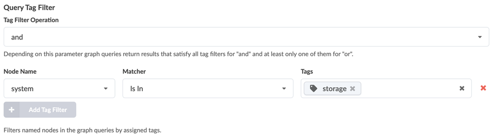
Query Tag Filter
Another useful customization option is the Query Tag Filter. Let’s say you tagged some switches in your blueprint as storage for a specific monitoring use case. You can configure this filter to perform the telemetry collection only on devices with the matching tag as shown in the following example:
Displaying the raw data from your custom telemetry collector shows only the raw data, so it may be difficult to conclude whether it signifies your network's normal or anomalous state. With Asptra, you are proactively notified when any anomaly is detected.
Performing Analytics
An IBA probe functions as an analytics pipeline. All IBA probes have at least one source processor at the start of their pipeline. In our example, we added an Extensible Service Data Collector processor that ingests data from your custom telemetry collector.
You can chain additional processors in the probe to perform additional analytics on the data to provide more meaningful insight into your network’s health. These processors are referred to as analytics processors.
Analytics processors enable you to aggregate and apply logic to your data and define an intended state (or a reference state) to raise anomalies. For instance, you might not be interested in instantaneous values of raw telemetry data, but rather in an aggregation or trends.
Analytics processors aggregate information such as calculating average, min/max, standard deviation, and so on. You can then compare the aggregated data against expectations so that you can identify whether the data is inside or outside a specified range, in which case an anomaly is raised. You might also want to check whether this anomaly is sustained for a period of time and exceeds a specific threshold. An anomaly is flagged only when the threshold is exceeded to avoid flagging anomalies for transient or temporary conditions. You can achieve this by configuring a Time_In_State processor.
Table 1 describes the different types of analytics processors.
|
Type of Processor |
Description |
|---|---|
|
Range processors Processor names: Range, State, Time_In_State, Match_String |
Range processors define reference state and generate anomalies. |
|
Grouping processors Processor names: Match_Count, Match_perc, Set_Count, Sum, Avg, Min, Max, and Std_Dev |
Group processors aggregate and process data before feeding into the range processors. These processors can:
|
|
Multi-input processors Processor names: Match_Count, Match_perc, Set_Count, Sum, Avg, Min, Max, and Std_Dev |
Analytics processors take input from multiple stages. These processors can:
|
For detailed descriptions of all analytic processors, see Probe Processor (Analytics) in the Juniper Apstra User Guide.
Multi-input processors are not supported for dynamic data types (dynamic text or dynamic number).
In the next section, we'll configure our BFD example probe to detect and raise anomalies.
Raising Anomalies and Storing Historical Data
-
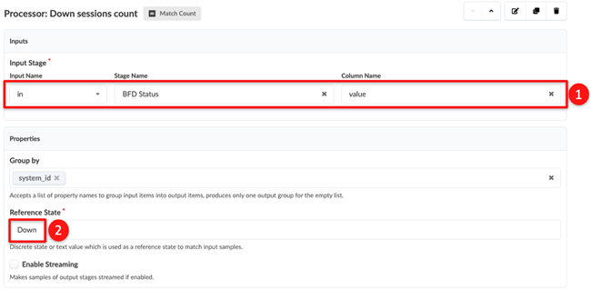
Configure the second processor, then Enter Down in
the Reference State field.
This processor configures the probe pipeline so that data from the previous processor is fed into each other.
 When you update the probe, the output shows the number of BFD sessions in the Down state by each device.
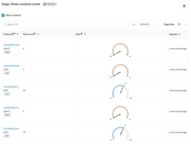
-
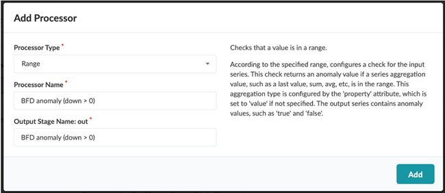
Click Add Processor, then select the Match Count
processor.
Give the processor a descriptive name (in this example, BFD anomaly (down > 0), then click Add.
-
Configure the third processor.
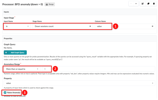
Enter the Input Stage – Stage Name, then select value for the Column name. In our example, we defined the stage name as Down sessions count.
Set the Anomalous Range to More than equal to and 1.
Click Raise Anomaly.
-
Click Update the Probe.
If you have any BFD sessions in the Down state, the probe generates anomalies for the BFD sessions.
-
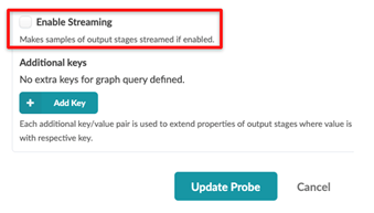
Check Enable Streaming in the probe
configuration.
-
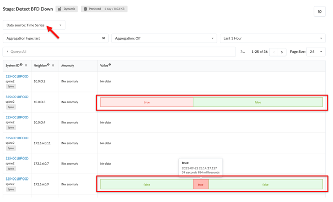
Finally, select the Data source: Time Series view to see the history
of changes in the data value monitored by this stage.