Jumpstart Juniper—Advanced

0:00 and bgp Concepts let's start by diving even deeper into

0:06 ospf Concepts by now you should be comfortable with configuring ospf

0:12 configured under protocols ospf you add an area number and then associate the

0:18 interfaces that are going to be participating in the ospf protocol

0:23 now within the interface hierarchy under ospf you can add additional options such

0:29 as the interface type so that you get rid of the Dr election especially if you only got two devices and you're running

0:36 a multi Access Link type such as Ethernet or setting a metric to specify

0:42 whether the link is more or less preferred but one of the big things that

0:48 cannot be overemphasized is the inclusion of the loopback interface as part of your configuration

0:54 one it's just great for troubleshooting and if you're using other protocols such

1:00 as ibgp or ipsec it's commonly used for tunnel endpoints

1:06 because the ospf interface can be used for multiple purposes It's Not Unusual

1:12 to see multiple IP addresses being added to the loopback interface and that means

1:18 when you go into ospf and you add the loopback interface that all of those

1:23 individual addresses will be added to your ospf database and distributed

1:29 throughout your network the way you can get around this issue instead of adding the interface name

1:36 under the interface configuration of protocols ospf add the IP address that

1:43 you want to have included in your ospf distribution

1:48 if working with a larger ospf Network you may find yourself in an environment where you have multiple areas in this

1:56 case you need to be aware of the area specific options and where they can be used when you can set up an NSSA area

2:04 and when it needs to be a stub area you also need to know things such as are you

2:10 going to be injecting a default route or are you going to do prefix summarizations these are some of the

2:16 things that you need to know we have talked extensively on how ospf

2:22 uses lsas to share information so each router can determine the best path to a

2:28 given destination the question is how does it do this well it uses the SPF

2:34 algorithm which stands for shortest path first now this is based on the dijkstra

2:39 algorithm which was used to find the best Loop free path between two points the way it works it starts with the link

2:46 State database which gets copied into a candidate database this candidate

2:53 database is processed by the SPF algorithm and produces a tree database

2:58 which holds these best routes now the SPF algorithm is run on a per

3:03 area basis on each router it's an independent calculation but it does

3:08 require that every router in an area have exactly the same picture of the

3:15 network now when it determines the best path and

3:20 it's stored in the tree database these results are passed to the junos routing

3:26 table the inet.0 where the route selection algorithm determines whether

3:32 the route will be marked active there are times when a network can

3:37 become unstable and during that period of time SPF has some built-in

3:42 protections to ensure that your processors are not overwhelmed with continuous processing of network changes

3:51 these rules state that if you have three consecutive SPF runs that there will be

3:57 a mandatory hold down Now the default time for this is five seconds but it can

4:03 be configured to be anything from 2 to 20 seconds and it's entered in milliseconds this helps keep the network

4:10 stable during periods of Rapid change not only can you set up your hold down

4:16 timer but you can set up the amount of time between any uh SPF run you can set

4:24 the minimum delay time this is done under protocols ospf SPF options delay

4:30 now this value can be set to anything from 50 to 8 000 milliseconds and it's

4:37 recommended that it at least be greater than the propagation time that it takes

4:42 information to get from one end of your network to the other

4:47 ospf has been around for a long time and because it has this has brought an issue

4:54 to bear on every modern day Network that uses ospf and the fact is is that back in the day

5:01 when ospf determined how it would Calculate cost it based it off of the

5:07 highest speed that was really around at that time which was a hundred megabits per second

5:13 so when it calculated a cost for any given link it was based off of a hundred

5:20 megabits per second and so everything over a hundred megabits a second would

5:25 end up with a cost of one at the time 1989 you know a hundred Megs

5:31 was a very high speed it wasn't thought of something that was just going to be blown away and barely existence like it

5:39 is today so when you're setting up your network you really need to change the reference

5:46 value that's going to be used within ospf now today the highest reference

5:54 bandwidth that you can set is a thousand gigs now again that's pretty high but

6:01 they thought a hundred Megs was high in the past I mean today the highest links

6:06 that we have today are 100 gigs 200 gigs even 400 gigs on Juno Juno's PTX so

6:13 we're well within those limits but the the definition of terabit interfaces are

6:20 being worked on even as we speak so you want to set your reference

6:25 bandwidth to a value that's high enough that should take you into the foreseeable future

6:31 now whether you want to put that as a hundred gigs or 10 gigs you know or a

6:37 thousand gigs I mean the higher you set it the more accurate it's going to be and helpful in the

6:44 future now you can set it on each device it is a per device setting that you can

6:50 do it's under protocols ospf reference bandwidth and you put in the value for

6:57 which you want the algorithm to calculate cost to be derived from

7:02 so again recommend one thousand now you can manually configure metrics yourself

7:10 so you can override the global by setting an individual metric as you can

7:15 see under the sonnet interface where it's manually being set to a metric of

7:21 12. an issue that you want to be concerned

7:26 about when managing costs throughout your network is you need to be sure that

7:32 it's implemented consistently on every device implementing cost Management on one

7:39 device and not on its other side that it's connected to can result in

7:46 asymmetric routing across your network so you want to be sure that the costs on

7:54 both sides of your link are always going to be the same unless you have a specific reason for doing otherwise so

8:02 be careful when managing your network costs whether you're using the reference

8:08 bandwidth or your individually setting leading costs be sure there's a consistency or as you can see on the

8:15 slide it would be very easy to result in asymmetric routing

8:22 let's move into a more detailed discussion about ospf areas

8:28 in today's networks it's not unlikely that you'll find a large-scale ospf

8:33 network that's running as a single area this is because interface links are much

8:40 more stable processors are much more powerful and gone are the days when an ospf area

8:47 could not exceed 50 routers today they are much larger than that

8:53 but there are other reasons why you may want to consider having a multi-area

8:58 ospf network and if you're going to do that then there are some specific area

9:04 types that are meant to help you uh control the size of your ospf database

9:11 these area types fall in four different categories stub totally stubby not so

9:18 stubby and totally not so stubby a stub area is used when you have a

9:24 section of your network whose only way out of that section is through the

9:30 backbone area of your ospf network in this case you can have one of two

9:36 different stub types either a stub area or a totally stubby area

9:42 now a stub area tells an ABR that any type phias that it sees from the

9:49 backbone do not need to be injected into that area either they do not need to get

9:54 to external routes or maybe there is other summarization that's taken place that they can get to those external

10:00 routes but they don't need all the individual external route entries

10:06 injected into their area so that can become a regular stub area

10:11 in a stub area you will see type 1 type 2 and type 3 lsas

10:17 and generally you'll see a default route that's injected to get to those external

10:22 routes if needed now in a totally stubby area it's just like a stub area except it says you know

10:30 what if I don't need a route to external

10:35 routes and there's a default route being injected well then I don't really need type threes because I'm just going to

10:42 send everything to the backbone the backbone will know how to get everywhere and this will reduce your database in a

10:49 totally so be areas to nothing more than type ones and type twos and this is

10:54 called a totally stubby area and it is again used when there's only

11:00 one way out of your local area and that is through the backbone

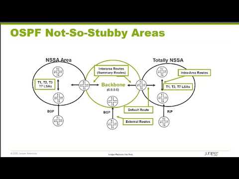
11:06 now the alternative to the stubby area is a not so stubby area

11:12 this is a situation when there is more than one way out of your network

11:17 however the majority of your traffic is through the backbone not through some

11:23 external connection that you have because most of your traffic is going to

11:29 travel through the backbone then what you want to do is kind of imitate what a

11:35 stubby Network did but we can't do that because a stub Network says no external

11:41 routes period so a not so stubby area lets us break that rule

11:47 we can inject external routes directly into our not so stubby area

11:53 however these routes will be marked as a type 7 not a type 5.

11:59 now a standard not so stubby area will have type ones type twos type threes and

12:04 type sevens but no externals from the backbone will be injected into this area

12:10 now it might be that NSSA area does have a connection to the outside world that

12:16 will give it its internet access and everything like that so I don't need any of the externals from the backbone

12:22 itself I can just do it directly I don't want to be sent through the backbone I'll take my direct connection that

12:28 might be one reason okay so that that that's an NSSA area but if I'm in the NSSA area and I'm

12:36 sitting there I'm saying look yeah I'm injecting routes in and for those specific routes I can take that route to

12:44 get out to them but everything else if I don't have a specific route for it I want to go

12:50 through the backbone so in this case in a totally not so stubby area we'll inject a default route

12:56 pointing to the backbone so they can get to their external lsas they can get to

13:03 other internal routers and for everything else they will use the default route that takes them into the

13:09 backbone and this is called a totally not so stubby area

13:14 now the main reason behind the stub area is that we want to reduce the number of

13:20 lsas that exist within our area to shrink the size of our database now a

13:26 stub area alone only says it only tells the ABR don't send me in don't allow

13:34 type fives to flood into my area and of course if type fives are not coming in I

13:39 obviously don't need type fours now how am I going to get to those routes that I've stopped coming in well

13:46 I can use a default route now in junos it requires manual

13:52 configuration from an administrator on the ABR to have the ABR inject the

13:59 default route into a stub area now when I have a stub area

14:08 then I really can't inject external routes into my area I can technically

14:17 redistribute routes locally but they will never go beyond my local router

14:23 so you really don't have an asbr capability with a stub area

14:29 and virtual links cannot Transit a stub area either so that's another feature of

14:37 a stub area when you decide to create a stub area

14:42 you're going to change how type fours and type fives flood throughout the

14:49 network in order to create an area as stub you need to configure all routers in that

14:55 area as a stub router this becomes an adjacency forming criteria

15:03 if you have multiple routers in an area all of them must be marked as stub

15:08 or else the router that is stub and the router that is not stub will not form an

15:14 adjacency when you create a stub area no default route is created by default if you want

15:21 a default route you must configure the ABR to tell it to inject the default

15:27 route into the stub area now let's look at how type 5 routes will

15:34 be affected so here we're injecting a external route into area 0 which is

15:41 creating a type 5 LSA these will then be flooded into area 2

15:47 and area 3. and then a Type 4 will be created by the abrs to be supportive of

15:54 the type 5. the stub area itself will not have any

15:59 type 4 or type 5 lsas injected even if external routes are set up in a

16:07 different area it will go ahead and create the type 5 LSA in that area they will be flooded

16:15 into areas zero they will be flooded over into area 2 but they still will not

16:21 enter into Area 1 in this example

16:28 foreign route in a stub area

16:35 well then you really don't need the type threes as well and you can further

16:40 reduce the size of the database by introducing the words no summaries into

16:46 your ABR configuration okay into your ABR configuration in this

16:53 way an ABR will say well you're a stub area so you don't need type fives and if

16:59 you don't have type fives you don't need type fours and then because you've added the no summaries we won't send in type

17:06 threes either now a stub area with no summaries is also called a totally stubby area but it

17:14 still does not by default inject a default route you still have to go through a manual configuration step

17:21 to ensure that a default route gets injected into this totally stubby area

17:28 now in this particular case you cannot have asbrs if you were to do

17:34 that you could always redistribute locally but it would never go beyond that route so why do it

17:40 and then secondly virtual links cannot Transit a no summaries area

17:48 when you decide to create a totally stubby area then every router in that

17:54 area must also be marked as a stub router this is an adjacency forming

18:00 requirements when one router is marked as stub any router that it will form an

18:06 adjacency with must also be stub now the reason behind stub is it stops

18:13 the creation of a type 5 being applied to that particular area we need to do it

18:20 on every router we do it on the ABR to prevent the type 5 from being injected

18:27 into the local area but we do it on the other routers so if they were to inject

18:32 a or try and redistribute a route into the area that it would fail that it

18:38 would not create a type 5 external and they would not be sent to any other routers so that's why every router must

18:45 be stubbed now on the edge we want to block the type threes from coming in so

18:52 we use the keyword no summaries that doesn't mean that the internal routers

18:57 cannot have type threes in fact if you put on a default route in the ABR and you tell it

19:05 to inject one into area three it will come in as a Type 3 and the other routers will process it just fine the

19:12 purpose of the no summaries that the ABR is to block the type threes from coming into the area from the backbone

19:20 now let's see what happens when we deal with type fives so now we have a router

19:27 in area zero that is an asbr injecting type fives

19:32 now the stubs will block it from going into Area 3 and area one but it will

19:40 flood just fine into area 2 which has no such designation

19:46 when configuring a stub area all routers in the area must be configured as stub

19:54 in the example shown on the slide there are two routers in area one router 2

20:01 which is the ABR and router 3 that is the internal router to area one now at

20:09 the top left here of our configuration we show the command to set router 3 as

20:16 stub in area one it's that area one stub and we can view that with the show

20:21 command that it is marked as stub we issue the same command on R2 which sets

20:29 it as stub now in this case we want our two to

20:35 inject a default route into area one so it knows how to get out to area 0 for

20:41 external routes and so R2 with the configuration of the

20:46 default metric command will inject the default route which will be an LSA type

20:53 3. in addition to that because after the default metric we put in the value of 10

20:59 the cost associated with that default route as it enters into the network will

21:05 be 10. in order to make an area a totally

21:10 stubby area follows the same commands that we saw on the previous slide except

21:17 on the ABR we're going to add the additional keyword no summaries

21:23 so we still specify the word stub if we want a default route which makes

21:30 sense we'll keep using the default metric and give it a cost value and

21:35 immediately following that we will add the keyword no summaries on the ABR only and it is this that

21:43 tells the ABR not to go ahead and flood any type threes into the local area

21:52 when configuring an area to be a not so stubby area or totally not so stubby

21:58 area there's some similarities and differences to a stub area

22:03 so first thing the similarities is that every router in the area is going to have to be configured as an NSSA area in

22:11 order to form adjacencies so that's like a stub except we're using NSSA this time when it comes to building

22:19 the default routes to configuring the default routes in the stub area all we

22:24 did was type in the default metric but now in The Not So stubby area we have to

22:29 use the keyword default LSA first before we can get to the default metric

22:35 and so when we configure a default route this way the default route will be injected into the ospf area in this case

22:44 Area 3 as a type 7 route now

22:49 another option that you have is that you add in the keyword no summary so now it's not a standard not

22:57 so stubby area it's a totally not so stubby area and now when you use that same command with the default LSA

23:04 default metric no longer will the default route be injected as a type 7

23:09 because it's now a no summaries it's injected as a Type 3 it's just the way

23:15 that it is now if you don't like the fact that you have this totally stubby area and it's

23:22 having a Type 3 and you really wanted it to be a type seven well Juniper has

23:27 provided a way for you to force it back to be a type seven and so in your

23:33 configuration when you've set it up to be a no summaries LSA you configure the

23:38 default LSA you configure the default metric and now you can force it back to be a type 7. now remember not so stubby

23:46 and totally not so stubby you cannot have virtual links to trade and satin a

23:51 not so stubby area looking at ospf flooding in an ospf

23:57 domain that hosts both stub and not so stubby areas we can see that there is no

24:03 impact on type 3 flooding they go everywhere however when a type 5 external route is

24:11 flooded into area zero we do see a change as this type 5 will not go into

24:18 Area 1 or area three but it will be carried into area 2 with the Type 4 LSA

24:25 being created now because Area 3 is an NSSA area

24:33 external route can get injected into this area as a type 7. when it hits the

24:39 ABR it gets translated into a type 5 in area zero

24:45 and then we'll go ahead and flood into area 2 but not area one

24:53 looking at the flooding patterns of stub and not so stubby areas that have been

24:59 marked with no summaries you see a big difference here now in the fact that no

25:04 type threes exist in these areas and then when external routes are injected

25:10 into the area then they are only going to be injected into the area that isn't

25:16 configured with these particular options in this case area two no additional type

25:22 5 show up No Type 4 show up in any of the areas if we still inject

25:28 routes into the not so stubby area the type 7 is created it is forwarded into

25:35 the backbone area and converted into a type 5 with no matching type four it's

25:41 unnecessary as we saw earlier and then this is carried over into area two so

25:46 you can see through the use of stub and not so stubby with no summaries we've

25:52 left our areas area one and Area 3 with a minimum of lsas to process by the SPF

25:59 algorithm while the use of stub and not so stubby

26:05 areas has done much to reduce the number of lsas in a non-backbone area it hasn't

26:11 impacted the number of lsas in the backbone area so we need to do some work on that we

26:19 can do that with the area range command that allows us to summarize routing

26:25 information it can be used in a couple of locations and here we see it used after the area

26:32 number in order to summarize type 1 and type 2 lsas

26:38 let's see how the use of stub areas and area range can reduce the number of lsas

26:45 that exist in both area 10 and area 0.

26:50 now pay attention to area 10 it currently is a regular area it is filled

26:57 with lsas and what we're going to do is we're going to make it a stub area

27:02 through configuration and the external routes will go away so we're going to lose both type fours and type fives

27:10 so we start by configuring the set protocols areas ospf 10 step on every

27:17 router in the area that means our 5 R6 R7 R8 and R9 will all be configured with

27:25 the same command stub and we reduce the number of lsas in area

27:30 10. we then come in and on the ABR only we add the command

27:38 default metric to inject a default route now because we now have a default route

27:45 and that's our only way out of the network I don't really need type threes so in that same configuration I can add

27:52 the word no summaries and now look we are down to just two types of lsas

27:59 within area 10. now this hasn't changed area zero

28:06 so if I go in and I add to my protocols ospf area 10 command the area range and

28:15 a prefix then this is going to summarize the type 1 and type 2 lsas that were sent in to

28:23 area 0. now remember originally every type 1 and type 2 I had

28:30 in area 10 resulted in a type 1 and type 2 summary in area Zero by using the area

28:39 range command now I get a single summary so I've reduced all those lsas in there

28:45 into a single summary now the area range is not just available

28:52 after the area number it's also available after the keyword NSSA and

28:59 this will go ahead and summarize type 7s now there's no option to summarize type

29:06 fives this command will summarize type sevens now we'll show you how using the NSSA

29:13 area designation and area range can reduce the number of lsas both in a

29:22 non-backbone area and a backbone area so we look over here at Area 51 Area 51

29:28 has Type 1 lsas type 2 lsas it has summaries from the backbone and it also

29:34 has type 5 externals that are being injected from this external route

29:39 now one of the first things that we can do is go ahead and configure this to go

29:45 ahead and be in the NSSA area now in reality just converting it into

29:51 an NSSA area didn't change the number of lsas that we needed to support it just

29:58 basically set up the type files or change the type fives to type sevens now

30:03 it did reduce over here the Type 4 in the backbone area so that is a little

30:09 bit of a savings but at the current time we haven't saved much in the way of lsas

30:16 so what we do is we go in and now we configure the NSSA area with a default

30:23 route so we're now going to inject the default route and if we inject the default route that means we don't need

30:31 the type 3 summaries anymore so we can go ahead and

30:36 add in the no summaries command and get rid of the type 3. so this reduces the

30:43 number of type threes in area 51. now it

30:48 hasn't done much for area zero so what we can do here is in order to get rid of

30:54 all the individual matches of the type 1 and type 2 Network lsas here that were

30:59 resulted in individual type 3 lsas over in the backbone area we can use the area

31:07 range command after the area number so this is going to change the one for one

31:13 count of summaries from type 1 and type 2s into an individual summary for the

31:20 type 3 reducing the lsas there the other thing is is that the type 7s

31:25 can now be summarized through the area range command after the NSSA and this

31:33 will reduce the number of type 5 routes that are converted that represent the

31:38 seven inside the area so here you can see that now our

31:44 backbone area just has their type 1 and type twos and a limited number of

31:49 summary and external routes that are coming in from the adjoining

31:54 non-backbone areas we're going to walk you through a demo

32:00 of ospf summarization we have two ospf areas area zero and area four area four

32:07 is a not so stubby area router 5 is injecting external routes

32:12 that need to be summarized into area zero and router 6 has many internal

32:18 networks that needs to be summarized into area zero our goal is to summarize

32:23 as many of the 172.160 through 9 24 routes without creating Rogue routes

32:31 Rogue routes are routes that you're advertising that you don't own so we can only advertise routes we own we want to

32:39 prevent the 172.16.9.0 24 route from being present

32:45 in area zero and we want to summarize both 172.28.0 through 3 and the

32:53 172.29 8 through 11 24 Networks

32:58 now for the purposes of this we're going to be just using three routers are 7 to

33:03 verify routes are in the NSSA area and are one to verify that summarization has

33:11 occurred and our ABR will be R4 and this is where we'll be doing our configuration

33:18 we'll start our demo on router 7. here we're going to look for the 172 16 16

33:25 routes to see yes we have all nine we'll do the same to look for the 28 routes

33:32 and we have them there and we're going to look for the 29 routes so in area 4

33:37 we have all the routes that we want to summarize in area zero let's make sure

33:43 they're showing up in area zero so we move over to router 1. and yeah we have all of our nine routes

33:50 in the 17216 Network we have all of our routes in the 28

33:55 Network and we have all of our routes in the 29 Network so we're fine so to summarize we

34:03 need to go to router number four or ABR and we need to summarize but we have to

34:09 figure out what is the best subnet to use so let's go ahead and just do our

34:16 um show route 10 essentially one seventy two

34:25 1.16 and yes here's our nine routes and we want to figure out the best summary and one of the tricks is you can play

34:31 around with your um you know prefix setting and here we

34:37 can see that a 20 still gives us all of our routes if I go ahead and add a 1 to

34:42 it okay well now I know that 20 gives me all of them 21 gives me a few less but

34:49 it's not um at the nine it doesn't stop at the nine so I know eight and nine won't fall

34:55 in a perfect boundary so if I can't do row grouts the only thing I can do is

35:01 zero through seven so let's summarize those and see what happens

35:06 so I'm going to go under protocols ospf area 4. now these are external routes

35:15 that we're dealing with we can tell that from the ospf preference of 150

35:22 and so what we're going to do is we have to put this in under NSSA if we just put

35:27 it in as an area range after area four then the type sevens wouldn't be summarized they have to be done under

35:34 after NSSA so I'm going to do 172

35:39 16.0.0 21 for my summary and now when I commit

35:46 okay it should summarize my routes and now when I go over to router 1 which is in area 0

35:52 and I look at my 16 routes yes indeed it did summarize them that it has all the

35:59 first zero through seven in one group eight and nine are independent routes which you may have to do if you do not

36:06 have a perfect summary boundary as part of your Networks

36:11 now we were told that we can't have nine in area zero so the way we can do that

36:17 with ospf is we still do an area range command

36:22 but we're going to identify the network and then use the

36:28 keyword restrict all right and we're going to commit that

36:34 and then we'll go look at R1 again and see if we've met our goal

36:40 N9 is gone so at this point I can ping 172 16 1.1 I can get through that way I

36:48 can do 4.1 get through that way I can do 8.1

36:55 but 9.1 will fail okay because we didn't let that host route come across or that

37:03 summary route come across now I'm going to show you something that's a little bit tricky when it comes to the

37:10 summarization you remember that we set up this big block of routes to allow well what if

37:18 you wanted to block a subset of those routes by trying to

37:24 throw in a restrict well if we go over to R1 and just test

37:29 this out and we try and ping 4.1 but we can still get there so if I got this big

37:36 block of permit I can't go in and restrict a subset of it however if we go

37:43 back here and we change things up and I take my 21

37:50 summary and I set it to restrict and then I go back to my four route entry

37:59 find it here here it is and what I'm going to do

38:05 whoops I want to delete the restrict

38:13 okay we can see the restrict is removed so

38:18 I'm committing this now when I go back over to R1 and I try and ping

38:26 1.1 I can't get to it if I try 2.1 I can't get to it because the block is

38:32 working however if I do 4.1 I can get there so it if you have a big permit you can't

38:41 block in the middle but if you have a big block you can permit in the middle just the way that it works just wanted

38:48 to let you know about summarization all right we've got a couple more to finish up in our Command here we need

38:55 to go ahead and summarize the 28 and 29 networks which are

39:00 internal not external so I'm going to do a set protocols ospf

39:06 area four but now I do not use NSSA if I did then the area range command wouldn't

39:12 work so I do area range 172 28

39:18 28.0.0 22 because there were four routes zero through three and then I'm going to

39:24 do the area range command but it's going to be for 29 and its

39:31 Network started at eight it was 8 9 10 11. so 8 22 and I'm going to commit

39:39 and now when I go over to R1 and I do a show route 172 28 Dot

39:49 zero dot zero slash 16. I only see the one route it's summarized

39:56 it if I go in and I do the 29 I can see it summarized that so

40:03 everything is working as it should and that's how ospf does summarization

40:10 we'll now move to bgp bgp is an EGP which stands for exterior

40:17 Gateway protocol this means it's not so concerned with how traffic moves inside an autonomous

40:24 system as how traffic moves between autonomous systems

40:29 in fact bgp is the core routing protocol that connects the internet

40:35 because you're connecting to other companies and you don't want them telling you how to route traffic through

40:42 your network bgp is all about control so there are many attributes available

40:48 within bgp that you can use through policies to provide this control

40:56 when it comes to calculating the best path bgp is a path Vector protocol

41:04 distance is determined by the number of autonomous systems that the traffic must Traverse to get to a destination not the

41:12 number of routers or the speed of the links now bgp supports two different methods

41:19 of Route Exchange there is the ebgp protocol that is used

41:24 to exchange routes between autonomous systems and there's ibgp that is used to

41:31 exchange routes inside an autonomous system if you're asking yourself if bgp is

41:37 right for you then you have to ask yourself another question and that is how are you connected to the outside

41:44 world if you only have a single connection to a service provider then you don't need

41:51 bgp you just need some form of manually created default route

41:57 if you're like customer a and you're multi-home to more than one service provider and you want to make an

42:05 intelligent decision as to which link to use to forward your traffic then bgp

42:12 might be your answer when setting up bgp peering there are

42:18 two types of sessions that could be created one is an ebgp session which is between

42:25 you and an external autonomous system these sessions are usually established

42:31 using the IP addresses of the physically connected interfaces

42:37 ibgp sessions are required when you have more than one bgp router inside your

42:44 network and need to take the routes received from one autonomous system and

42:49 pass it to another router in your network ibgp sessions are usually established

42:56 between the loopback addresses this allows you to maintain connectivity

43:01 even if you were to have a physical failure on the connecting links

43:08 bgp uses five different message types in order to communicate there are open

43:15 messages keep alive messages update messages notification messages and

43:21 refresh messages bgp uses open messages to establish

43:27 peering relationships between manually defined peers since bgp relies on TCP

43:35 for Reliable connections a TCP connection must be established first

43:42 once TCP has established connectivity bgp will send open messages to confirm

43:49 the neighbor identity and set up an established relationship between the two

43:55 peers bgp uses update messages in order to

44:01 exchange learned information between bgp peers some information is required and will

44:08 appear in every update message this includes an lri which stands for Network

44:14 layer reachability information and for standard ipv4 and IPv6 bgp

44:22 this is for prefixes other fields that are mandatory include

44:27 origin as path and bgp Next Top bgp also contains some optional fields

44:35 that may or may not be included in any given message this includes local preference Med and

44:43 communities EGP may also use an update message to

44:48 withdraw information that has been previously sent the other messages used by bgp are keep

44:57 Alive's notifications and Route refresh keep the lives are used to maintain bgp

45:04 sessions you set the keep alive time through the configuration of the hold time option

45:10 and this hold time option is three times the keep alive interval which means if

45:17 you take the default hold time of 90 seconds and divide it by three then keep

45:23 alive will be sent every 30 seconds you do not directly configure the keep

45:28 alive timer you define the hold timer and keep the lights are sent every one

45:34 third of that time period notification messages are bgp's error

45:41 messaging system so whenever an error is detected within a bgp session such as a hold timer

45:48 expiring or a change in neighbor capabilities a notification message will

45:54 be sent and the route refresh is used to ask a bgp peer to resend all routes of a

46:02 specific address family as new routes are learned and added to bgp they are placed in bgp updates and

46:11 forwarded to other bgp peers in order to prevent Loops these updates must follow

46:17 several rules rule number one ibgp learned updates can only be forwarded to

46:24 ebgp peers rule number two states that ebgp learned updates can be forwarded to

46:30 both ebgp and ibgp peers and rule number three says ibgp Loop prevention requires

46:37 a full mesh design so let's look at that in our example on the slide as a new route is added to

46:45 router number one it's placed in a bgp update and forwarded to router number two using ibgp

46:53 router number two follows rule number one ibgp learned routes can only be forwarded to ebgp peers so router number

47:01 two forwards it to four four receives it and follows rule number two ebgp learned

47:07 routes can be forwarded to ebgp and ibgp peers for this example we're going to

47:14 say that for only peers with routers 5 and routers 6 using ibgp

47:21 so when five receives the route it follows rule number one ibgp learned

47:27 updates can only be forwarded to ebgb peers and the same goes for router

47:32 number six so the question is how is 7 going to

47:38 receive the update to forward it to its ebgp pair and the answer is well five can't break

47:46 the rule of number one because if five could send it to seven seven could send

47:51 it to six six would send it to four and that would be a loop so this is where

47:57 rule number three comes into play ibgp Loop prevention requires a full

48:02 mesh design so the way 7 gets the update is four must send it directly to seven

48:08 through its own pairing so this is the way that bgp update rules are applied

48:16 in addition to having different forwarding rules ibgp and ebgp process

48:22 updates differently ebgp updates change the aspath and bgp

48:28 next up while ibgp updates do not change anything by default

48:33 now while there are differences they also have something in common a bgp router will verify Next Top reachability

48:40 before adding the route to the routing table we will now walk you through how bgp

48:47 updates are processed as they move from router to router now in our example

48:53 router number one is adding a new route into bgp and sending it as an ibgp

49:00 update to router number two so router number one is creating this brand

49:06 new and so it looks at the bgp update says I have to add an nlri which will be

49:12 the prefix I have to add an origin I learned this from my igp

49:18 then I go ahead and add an as path which right now it's never left the borders of

49:25 an autonomous system this is an ebgp thing so it's left at null and my bgp

49:31 next top is the router that added it into bgp in the first place and so we

49:37 see the 192.168 1.1 now when router number two receives this

49:43 update the very first thing it must process is can I get to the bgp next top since it should be peering with one

49:50 through its loopback and that is the bgp next stop there should be no problem getting to the bgp next up the route

49:58 gets accepted now router number two is going to send it as an ebgp route to

50:04 router number four so it needs to follow the processing rules of ebgp which says they're going

50:11 to change the as path and the bgp next top so when we look at the next bgp update

50:17 message that's going to flow between 2 and 4 the nlri will be the same the

50:22 origin will be the same but the ebgp processing will add the as path of the

50:29 autonomous system number that it's leaving in this case number 10. it will

50:35 also change the bgp next hub to be the peering address that is assigned to four

50:41 and that's going to be 1.1.1.1 and this is the address that's going to be sent in the update message

50:48 now when this update message gets sent to four the number one thing that the

50:54 router 4 does say can I get to the bgp next top since it's a directly connected

51:00 link there should be no problems the route gets accepted and then four processes it for forwarding Now it only

51:08 has ibgp peers so it's going to not change anything by default

51:14 so here the nlri is 203.8 the origin is one the as path stays the same and the

51:21 bgp next top is still at 1.1.1.1 and this is the number one reason why bgp

51:28 will break inside an autonomous system because we don't normally add an

51:34 exterior Network into our igp so in order to fix this problem the most

51:41 common way it's done is through a process called Next Top self where we actually take some extra action and

51:48 configure router 4 to change the bgp next top

51:53 to configure bgp there's a couple of sections in the Juno's hierarchy that

51:58 you're going to have to configure the first is under routing options where you define the devices assigned

52:06 autonomous system number now autonomous system number come in two formats a two byte format and a four

52:12 byte format the reason why we have a four byte format is we've run out of two byte numbers because in a two byte field

52:18 the largest amount that you can have is 65 535. now within the two byte number

52:27 range some of them are public and some of them are private so the numbers

52:34 64512 through 65535 are considered private you can use them your service

52:41 provider can assign them to you they should not be advertised out into the

52:47 internet themselves but other than that they can be used freely

52:56 private numbers are assigned by Ayanna and so you'll need to apply for those

53:01 there's a cost and there's a justification that you have to make in order to be assigned a uh public

53:08 autonomous system number now to configure bgp we go under protocols bgp

53:16 and because there's two types of bgp when we create our bgp groups we have to

53:22 Define if it's an ibgp or an ebgp so that traffic flows can follow the

53:29 forwarding rules and processing requirements that we've talked about earlier

53:35 so our first group here we're showing is an ibgp group we're giving it a name

53:40 we're defining it as internal the local address is used to overwrite

53:46 the routing engines innate desire to create packets using the IP address of

53:54 the egress interface as the source address and if that's the case when it gets over

54:00 to the peer the peer will not recognize you because you're peering between loopbacks so adding the loopback address

54:07 field basically tells the routing engine to use this as the source address of any

54:14 bgp messages that are sent so they'll know it's coming from a trusted peer

54:20 you also have to Define their address that you're appearing to within the

54:26 configuration of the group and again it serves two purposes it is the

54:31 destination address that's used to send the message over to the peer but it also

54:38 acts to confirm that the messages you're receiving are from authorized peers

54:45 when you want to create your ebgp group you give it a group name

54:50 type in the type which is is it ebgp or ibgp it's not really necessary to

54:57 include the designation external except it's considered best practice

55:03 because external is the default you then Define the pure as of your peer

55:09 and the neighbor IP address of your peer now again that neighbor IP addresses does two things one it is the

55:16 destination address that's used when you send bgp messages but it's also used to

55:23 confirm that you're receiving traffic from authorized trusted peers

55:29 with bgp configured and peering relationships established bgp can now

55:36 receive update messages these update messages carry routes that need to be

55:42 added to the routing table and the best route will need to be chosen

55:47 unlike igps that use cost to select the best route in bgp there are many

55:53 attributes that can be used to make the choice these attributes are processed in a

56:00 specific order and are listed in the bgp route selection summary table on the

56:06 slide the first criteria is to look at the local preference this is an optional

56:12 value carried in bgp update messages where the higher value is better in fact

56:19 in the bgp route selection process this is the only option where higher is better

56:25 if the local preferences are the same then it moves to the next attribute to

56:30 evaluate the next attribute is the as path and it's looking for the route with the

56:37 shortest as path length if they are both the same then it moves

56:42 to the next value which is origin code now the origin code is learned at the

56:49 time a route is added into bgp and never changes in this case the lower value is the

56:57 chosen route if they are the same then it moves to What's called the med the

57:02 multi-axis exit discriminator it wants the lower Med if that's the same then it

57:10 prefers routes learn from an ebgp peer over an ibgp peer

57:15 now the reason for that is that an ebgp peer will get it out of the local

57:22 network faster and use less internal bandwidth

57:28 if they're both ibgp peers then it moves over to number six where it prefers the

57:34 path whose next hop is resolved by the igp route with the lowest igp metric

57:40 now if those are the same then it looks at cluster length which is used in an environment that uses route reflectors

57:47 if route reflectors aren't used then it moves to the next one where it prefers routes from the pier with the lowest

57:54 router ID and if the routes are re being received from the same router then it moves to

58:00 the last option which is to prefer routes from the pier with a lower peer IP address

58:07 the bgp route selection process is designed to produce a single route to be added to the route table

58:14 this route will be the only route used by the system even when there might be more than one possible path

58:20 when the router ID or peer ID are the decision criteria as to which of these

58:25 paths to choose you can add the keyword multi-path to the bgp configuration

58:32 this will cause bgp to ignore these last two comparisons and consider both paths

58:38 as possible and will load balance on a per prefix basis across both links

58:44 shown here are three possible scenarios where multipath could be used

58:49 in scenario a you have two different pairing sessions to the same router

58:55 in scenario B you have two different pairing sessions each to a different router but these routers belong to the

59:02 same as and in scenario C you have two different peering sessions each to a different

59:08 router but these routers are part of different autonomous systems in this last scenario you must add multiple as

59:16 to the multipath option in order to provide the load balancing functionality

59:22 um in the example on our slide you see a bgp peering to two different neighbors

59:29 that are sending this router the same routes multipath is not configured

59:36 when we look at the show bgp summary command we can see that four routes are

59:42 being received from each peer but the routes from the lower peer ID are being

59:48 selected as active and we look in the routing table we see that the bgp active

59:56 route is only showing one next hop by adding multi-path to the

1:00:03 configuration we can see now with our show bgp summary command that routes

1:00:08 from both peers are selected as active and when we look at our routing table we

1:00:14 can see that there are two Next Tops per active route however by default the

1:00:20 forwarding table maintains just a single Next Top per route if we want to do load

1:00:25 balancing per flow we would also need to add a load balancing policy

1:00:33 up to now we have been configuring ebgp sessions using the IP address of the

1:00:40 directly connected peers and this is how it was designed to be built

1:00:45 but with the availability of ethernet and the reduced prices of links

1:00:52 redundancy has come into play and ebgp users want to have more than one

1:00:59 connection when there's more than one connection between two devices

1:01:05 ebgp sessions can be configured to peer with non-physical addresses and load

1:01:12 balance across the links in our example R1 wants to appear to the

1:01:18 loopback of R2 and R2 wants to appear to the loopback of R1

1:01:24 now in order for this to happen R1 has to know how to get to the loopback of R2

1:01:30 without getting the route from bgp so a static route is required and in this

1:01:37 case we want more than one link so we can load balance across the two paths

1:01:44 now to tell ebgp that it is no longer going to be a directly connected

1:01:50 connection we can go ahead and configure multi-hop

1:01:56 now when you turn on multi-hop it allows bgp to change the TTL to 64 and thereby

1:02:06 it can make a connection to a device that is not directly connected

1:02:12 for security purposes you can reset the time to live to 1 which would be allowed

1:02:19 for a directly connected device that is to its loopback because

1:02:25 junos does not update the time to live until it leaves the box and since the

1:02:32 traffic gets to the box and it's just an internal interface the time to live will

1:02:38 not be increased and so A Time To Live of one will allow it to connect to the

1:02:43 loopback of a directly connected device in our configuring bgp demo we have

1:02:49 created two autonomous systems as10 and as20

1:02:55 we'll be configuring R2 R2 will establish an ebgp pairing to R4

1:03:02 using the directly connected link R2 will establish an ibgp pairing to R1

1:03:09 and R3 using their loopback addresses so let's get started

1:03:16 before we can configure bgp bgp relies on TCP in order to establish

1:03:23 connectivity so we need to test our TCP reachability to our peers

1:03:28 so we'll start off by doing a ping of our ebgp

1:03:34 peers interface because that's directly connected that should be the most easy

1:03:39 one to prove and so yes we do have connectivity and now we need to confirm

1:03:45 reachability to the loopback of our peer so we want to ping the loop back

1:03:51 and while I could just do the loopback this would be my ability to reach them then I would have to connect to them and

1:03:57 make sure they can reach back I'd like to test both at the same time which I

1:04:03 can do by changing the source address to my loopback

1:04:09 and so now when I change the source I'm not only testing my ability to reach the peer but the peer's ability to reach me

1:04:16 and so I can reach our one our one can reach me let's do the same with R3 yes

1:04:23 everything is working fine so we're now ready to start configuring bgp

1:04:29 so we need to be in configuration mode now the first thing I want to do is I

1:04:34 need to set my autonomous system for my device and this is done under routing options

1:04:41 and here I set up my autonomous system which is going to be 10.

1:04:46 now once I've configured that I'm ready to start configuring my bgp group

1:04:52 now to configure ibgp we need a few things so set protocols bgp and I'm

1:04:58 going to name a group and I'm going to do it for ibgp whoops

1:05:05 ibgp and so the next thing I need to do is tell the system that it's going to

1:05:11 follow the forwarding rules of ibgp so I say it's a type internal group an ibgp

1:05:16 group I then need to tell it my local address this will put in the source i p address

1:05:26 of the packet cre engine sends so they will know that it's an approved peer so

1:05:31 I'm going to type in my local address of 192 168 1.2

1:05:41 all right so I've typed in my local address

1:05:48 okay now what I need to do is type in my peers address so set protocols bgp

1:05:56 Group ibgp by the way I could have changed the hierarchy level in order to

1:06:04 prevent me from having to retype in everything again but I don't mind typing

1:06:09 in the commands gives me good practice and my neighbor is 192 168 1.1

1:06:17 and I also have 1.3 for Neighbors so let's look at our configuration again

1:06:24 and see if we've forgotten anything and we have our type we have our local

1:06:29 address we have our neighbors and this is all we need to do a basic ibgp

1:06:35 connectivity so let me do a commit and then let's see if our bgp peering

1:06:43 comes up so run show bgp summary this is the command I

1:06:49 like to do and I can see my peerings are up and what we're looking for is this established

1:06:56 on this screen here you can see it over here on the right

1:07:03 here right established all right so we do have our established

1:07:09 state we're not receiving any routes which we could see down here if we were

1:07:14 okay but we do have an established peering relationship so now we need to

1:07:19 appear with our ebgp peer we kind of follow the same rules we do set

1:07:25 protocols bgp we create a group so we can Define the type of pairing

1:07:32 relationship it will be we'll call this ebgp it will be type external

1:07:39 now here the only thing I need to do is to find the peer as which is 20.

1:07:45 and the neighbors IP which is 172 16 0.1

1:07:52 I commit that show protocols bgp so you can see the

1:07:58 group configuration that we did and now I do a run show bgp summary and

1:08:06 see I can see that we're up this is my peering

1:08:12 for the ebgp peer I can see that the as number is different from mine we're not

1:08:20 receiving any routes but we are up and running with bgp

1:08:26 in this section we'll talk about bgp attributes and policy since bgp is all about control it's good

1:08:34 to know that bgp behavior can be influenced by policy bgp attributes can be matched or changed

1:08:41 using import or export policies and you can differentiate between ibgp and ebgp

1:08:47 routes bgp stores routes and three main rib memory tables there is the ribbon that

1:08:54 stores all received routes from a bgp peer rib local stores routes that the

1:09:01 local router uses to forward traffic and the rib out that stores all routes that

1:09:07 are going to be advertised to peers Now by default only active routes in the

1:09:13 local routing table are advertised and specifically the single best route is

1:09:19 the one that gets advertised now if you have a bgp route that is

1:09:25 overshadowed that means one that has a identical route but a better preference

1:09:31 which makes the bgp route inactive that route will not be advertised to a bgp

1:09:38 peer unless you configure the option advertised and active

1:09:45 bgp import policies are processed after the routes have been received from peers

1:09:53 and stored in the ribbon table the import policy takes the information in the ribbon table filters anything

1:10:01 that's supposed to be dropped manipulates whatever attributes are supposed to be manipulated and then

1:10:07 sends it to the IP routing table where it's then processed to determine

1:10:14 what the best route is to send to the forwarding table this slide will cover how import

1:10:20 policies are processed when routes are received in this case from as1 and as3 they are stored in the

1:10:28 ribbon table the import policy will then go through the ribbon table and apply whatever

1:10:35 rules have been set up in this case the zero zero route from as1 should be

1:10:43 rejected in which case junos will go back and mark that route in the ribbon

1:10:48 table as hidden next the import policy says to prefer

1:10:54 the 192.168.14.024 from as1 and accept all

1:11:00 as3 routes so we'll take that information and move the appropriate routes making any required changes and

1:11:07 place them in the routing table here is where the choice of the best route is decided upon and forwarding

1:11:15 information is determined and that information is used to update the forwarding table

1:11:22 now if you want to look at the rib end table there is a command you can use to do that there's a show route receive

1:11:28 protocol bgp where you establish the peer ID and now you can see the ribbon

1:11:34 table showing you the routes that you have received now when you execute this

1:11:40 command you will not see any routes that have been marked as hidden so after the peer ID you can add in the keyword

1:11:47 hidden to view those routes as well now if you want to view the results of

1:11:54 your import policy after your import policy we'll want to look at the IP routing table and so here you can use

1:12:02 the command show route protocol bgp Source Gateway with the peer ID and you

1:12:08 will see those routes in the routing table after the import policy has been

1:12:14 applied in junos bgp export policies are applied between the rib local which is your IP

1:12:21 routing table and the rib out tables which is where changes and modifications

1:12:27 are stored before they're sent to the actual bgp peers

1:12:32 this is an example of how junos processes export policies we start with

1:12:38 our main routing table that contains all the routes and we apply the rules that exist within our policy here we say do

1:12:46 not send a default route send the 192.168.14.024 to as2 with a metric of

1:12:53 10. do not send the 192.168.27.024 to as4 and send the

1:13:00 aggregate for local routes so these rules are applied to the existing

1:13:06 routing table and the results are copied into the rib out table

1:13:13 from the rib out table the appropriate routes will be set to the bgp peers

1:13:20 now to view the rib out table you can use the show route advertising protocol bgp with the peer ID to see the routes

1:13:28 that were actually sent what makes btp so powerful is its

1:13:34 ability to use attributes to control traffic flow this makes attributes very

1:13:39 important to the whole operation of the bgp protocol attributes can be used to decide if

1:13:46 routes will be accepted from or advertised to other bgp peers attributes can be altered in an attempt

1:13:53 to influence the routing decision of a neighbor now attributes fall into one of four

1:13:59 categories well-known mandatory well-known discretionary optional transitive and optional non-transitive

1:14:07 so well known basically says that every implementation of bgp that exists must

1:14:14 know of this option so every bgp router must know how to

1:14:20 implement origin must know about as path must have a bgp update and know how to

1:14:29 work with it now it could be mandatory so in this case this would be your

1:14:36 origin as path and bgp Next Top it could be discretionary such as local preference every bgp implementation has

1:14:44 to know about local preference but they don't have to use it in every bgp update

1:14:49 optional means that someone who writes their bgp code doesn't necessarily have

1:14:55 to know about this option or be able to process it and if that's the case then

1:15:01 this optional will either be defined as transitive or non-transitive transitive means it can be passed beyond

1:15:07 my local as and non-transitive means it cannot one of the well-known mandatory bgp

1:15:15 attributes is the bgp next top this must be supported by all bgp implementations

1:15:20 and included in every bgp update this only makes sense as the bgp next

1:15:26 top must be verified as reachable every time a bgp update is received

1:15:31 now if it's not depending on whether it's an ibgp update or an ebgp update

1:15:37 the route could either be marked as hidden or potentially even discarded

1:15:42 Now by default the bgp next top attribute is only modified when

1:15:48 advertised across an ebgp session but it can also be modified by policy and is

1:15:54 often used to fix the problem in an ibgp session environment where the bgp nexop

1:16:02 needs to be changed there is an issue with bgp next hops

1:16:08 that needs to be considered in your bgp design this is due to the fact that ebgp and

1:16:15 ibgp updates are handled differently in our example when as2 sends an ebgp

1:16:22 update to R1 it changes both the as path and the bgp next hop it's going to set

1:16:29 the bgp next top to the interface address that connects R3 and R1 so it

1:16:36 will now be 10.2.2.2 when R1 receives it it's going to create

1:16:43 an ibgp update and send that ibgp update packet to R2 but it doesn't change the

1:16:51 bgp next top so when R2 receives it it's still 10.2.2.2 it does a recursive lookup

1:16:59 can't find that route in its routing table and so it marks that route as

1:17:05 hidden and will not use it the way to fix this problem is to make

1:17:11 sure that R2 knows how to get to the bgp next top

1:17:16 two ways you can do this the way shown on the slide is we go into protocols ospf we take the egress facing interface

1:17:25 the one facing to as2 place it into ospf as a passive

1:17:31 interface so now R2 will know about that Network and be able to resolve it when

1:17:37 it does its lookup and the route can become active another solution not shown here is to

1:17:43 change the bgp next top on R1 and set it to itself or to the peering address that

1:17:51 R2 peers to so R2 will know how to get to that next top

1:17:57 a commonly used bgp attribute is local preference it's both well-known and

1:18:02 discretionary so it must be supported in all bgp implementations but it's not required to be in every bgp update

1:18:10 now a bgp local preference attribute is only used within an autonomous system

1:18:16 it's never advertised to an ebgp peer and it's used to control which exit

1:18:21 traffic will use to leave the autonomous system in local preference a higher value is

1:18:28 more preferred and it's used as the first tie breaker in the bgp route

1:18:33 selection algorithm the default value in junos is 100 and

1:18:39 when set it is always advertised to an ibgp peer

1:18:44 in our local preference example we start off with as2 advertising a route into

1:18:50 as1 to reach 10.8.8.0 R3 is receiving two copies of this route

1:18:58 and needs to decide which one will be the more preferred going through the

1:19:03 standard bgp route selection process it will fall down to the point where it

1:19:09 gets to the lowest router ID which is from R1 and that will be the more

1:19:14 preferred route to establish control over that

1:19:19 decision-making process the local preference can be modified

1:19:24 now here we're going to R1 and we're going to make the route that R1

1:19:31 advertises to R3 less preferred by setting the local preference to a lower

1:19:37 value and applying it as an ibgp update from R1 to R3 as an export policy

1:19:46 this same thing could have been done on R2 but making it a higher local

1:19:51 preference than the default value of 100 so it can work in different ways but

1:19:58 achieve the same results with the policy being applied when we go back in and do

1:20:04 our show route protocol bgp for the 10.8.8.0 24 route we can see that the

1:20:12 higher preference value of 100 makes the R2 route now more preferred over the R1

1:20:18 route another well-known mandatory apgp attribute is the as path so it must be

1:20:26 supported by all bgp implementations and included in every bgp update

1:20:32 now the as path consists of a list of the as numbers that the update has passed through and that a packet will

1:20:39 need to Traverse to get to its destination by default the as path will be modified

1:20:46 when advertised across an ebgp link the as path serves multiple purposes in

1:20:52 bgp first it is used for Loop prevention when a bgp update is received the as

1:20:59 path is checked to see if it contains the local as if it does the update is considered a

1:21:04 duplicate and the update is ignored the as path is also part of the bgp

1:21:10 route selection process it is checked immediately following the local preference to determine whether or not

1:21:17 the route is the best for a given prefix if the as path of the route update is

1:21:22 shorter than the other routes then this route will be considered best and become active in the routing table

1:21:30 aspath can also be used to influence incoming traffic by using policies to add additional

1:21:36 local as paths to some routes they become less preferred so other external

1:21:42 routers will prefer a different path in policies and some show commands regex

1:21:49 can be used to parse an as path junos includes a powerful pattern

1:21:54 matching engine to process regex statements it can work on fixed strings

1:22:00 which is needed for as paths and on variable patterns of text used for

1:22:05 Community matching regex works with a combination of text

1:22:10 and special operators and can perform context-sensitive matching

1:22:16 this is an example of how aspath can be used to control incoming traffic

1:22:22 as1 is sending routing updates to as2 and as3 and they are forwarding it to

1:22:29 as4 now as1 would prefer if as4 sent traffic

1:22:34 through as3 unless as3 were down and then it can use as2

1:22:41 how does as1 communicate with as4 and say hey I would prefer this

1:22:47 well the way as1 can do this is doing what is called negatively biasing

1:22:53 another as this means we want to make as2 appear to be a less preferable path

1:23:00 from the perspective of as4 as one can do this by writing a policy and then

1:23:09 this policy we use the aspath pre-pen command where we say to add our own

1:23:16 autonomous system number two more times than the normal EGP update process would

1:23:23 do as2 will receive that and forward it to

1:23:28 four and four should now prefer three so let's look at that so once as1 takes this policy and

1:23:36 applies it to the peering it has with a neighbor 2. then routing updates sent to as3 will be

1:23:45 the normal ebgp process where it places the current as number into the as path

1:23:53 as it forwards it it sends it to three when three wants to send this route to

1:24:00 as4 it puts it in an update and pre-pins its own as number so when it arises four

1:24:07 there are only two as entries in the as path now when as1 sends its route update to

1:24:17 as2 the ebgb process puts in the as number and then the policy adds that same as

1:24:24 number two more times in the aspath list when as2 receives it it thinks that it

1:24:32 already has gone through three sites as there are three individual as path

1:24:38 entries in there and it will go ahead and forward that route now to as4

1:24:43 pre-pending its as number and including the three as number entries that were

1:24:50 sent from as1 now when as4 has these two routes and it

1:24:56 goes through the route selection process as path being the second one it's going

1:25:01 to prefer the path through as3 and that's where it will direct its traffic

1:25:07 another bgp attribute that is a well-known mandatory

1:25:13 must be included in every bgp update must be known by every device is origin

1:25:20 the origin value is installed by the originating router and indicates how

1:25:26 this route was learned there are three origin codes there's I

1:25:32 for internal e for external and question mark for incomplete

1:25:38 whenever in junos you redistribute a route into bgp it will get the origin code of I this is

1:25:46 the Juno's default and the only one that Juniper uses there is an E when the route is learned

1:25:53 from EGP but EGP is a dead protocol it was the precursor to bgp and it's no

1:25:59 longer in use and some vendors do use incomplete when they redistribute routes

1:26:05 into bgp now you can see the origin code of a

1:26:10 route when you view it it will always be to the far right of the as path

1:26:17 now origin as an attribute is rarely used it's out there it could be used but

1:26:24 it's rarely used so we'll move on to our next attribute the next bgp attribute to discuss is

1:26:32 called the med or the multiple exit discriminator it's an optional

1:26:38 non-transitive attribute which means that every bgp implementation does not

1:26:43 need to understand it or in fact even use it Med is never passed through 1as to

1:26:50 another by default junos only Compares Med values on routes that come from the same

1:26:57 as and it informs neighboring ass's which

1:27:02 Ingress path to use to reach the local as the lowest value is best and by default

1:27:09 is based on the igp metric in our example of Med

1:27:17 R3 injects a new route into bgp and those routes get forwarded to R2 and R1

1:27:25 the internal link costs of R3 to R1 is 10 and the internal link cost from R3 to

1:27:33 R2 is 1. now this med value would be forwarded to

1:27:39 as2 and because the metric value becomes the med value R4 sees the path through

1:27:46 R2 as being the better path walking through the routing tables are

1:27:54 three forwarded this route to both R1 and R2 R1 has a cost of 10 R2 has a cost

1:28:03 of one and if we look over on R4 and we look at that route we can see that r2's

1:28:11 metric became the med for the advertised route and the R1 route the metric became the

1:28:20 mid since the lower Med winds R4 has selected the path through R2

1:28:29 by writing a policy on R2 so that when the 203 route is advertised to the ebgp

1:28:37 peer we set the metric to 100 that makes it much larger than the metric value

1:28:45 that previously was on R1 when we export that to our bgp peer then

1:28:54 what we'll notice is that the R2 path now has a med value of 100 and our R1

1:29:02 path has the original Med of 10 but it's more preferred because now it's lower

1:29:10 another commonly used attribute is community now Community is an optional transitive

1:29:19 attribute that is not required to be understood or used but must be

1:29:25 advertised to all peers it's great for helping you organize groups of

1:29:31 destinations that share a common property it can help you simplify your routing

1:29:37 policies by identifying routes based on their logical bounds that you establish

1:29:44 trying to match on as numbers is very broad because there's lots of routes and

1:29:51 trying to match on IP prefix to manage your network is very granular because

1:29:56 then you need to have lots of Route filters so communities can be used by themselves

1:30:03 or can be used with other attributes to accept prefer or advertise bgp route

1:30:13 there are a lot of things that you can do with communities the more you know

1:30:18 about them the more effectively you can use them in your network because communities establish categories for

1:30:25 routes and prefixes they're often used by service providers to allow you to communicate with them so

1:30:32 that they can set local preference on routes rather than you having to manipulate Med

1:30:39 communities can be used to cut down on manual reconfiguration and complexity of

1:30:44 maintenance jobs if a new prefix is placed in a community no other changes to routing policy are

1:30:51 necessary because it will be recognized by the community and the appropriate policy rules will take effect

1:30:59 however too many communities require more manual maintenance and too many

1:31:05 overlapping communities can be a nightmare to manage

1:31:11 there are two types of communities there are well-known communities these

1:31:17 are communities that everybody agrees on how they will be used and they have Global meaning there's not many of them

1:31:23 we'll discuss those on our next slide and then there are local used communities which are communities you

1:31:31 define for your own use they have whatever meaning you want to give them

1:31:37 a community itself is a four octet value

1:31:43 there are two high order octets that represent an as number

1:31:48 of which the maximum value is 65535 and then there are two low order octets that

1:31:56 represent some value that's unique to that as which again the maximum value is

1:32:02 six five five three five now a route can belong to many

1:32:08 communities and this would be stored as a community attribute

1:32:14 so the community attribute can have many communities in it so a community

1:32:20 attribute is a list of these four octet communities that are these individual

1:32:26 Community attribute values and they get associated with a route

1:32:32 now when you define a community there's two high order octets there's the two

1:32:39 low order octets they are separated by a colon and you can see an example on the slide

1:32:46 of the as number now when you're setting up the as number just know that as0 and

1:32:54 as65535 are reserved numbers and cannot be used in your local use communities

1:33:02 now because as numbers come in two forms the two bytes and the four bytes if you

1:33:08 are using a four byte as number and you want to configure that in your community

1:33:15 string then what you need to do is type in your long as number your four byte as

1:33:23 number and end it with a capital l

1:33:28 now four byte asns can also be represented using a format of two

1:33:36 two byte numbers separated by a period

1:33:43 there are three well-known communities however because confederations are

1:33:48 rarely used today though only the two main ones no export no advertise are

1:33:55 widely used now no export is used to limit routes to

1:34:02 be distributed within that as but no farther no advertise means that the routes must

1:34:09 not be advertised to any other bgp peers

1:34:14 so if I'm an ebgp router and I attach the no export Community as I send it to

1:34:22 my neighbor they will not be able to advertise that route beyond their borders

1:34:30 if I add the no advertised well-known Community to a route that I send to an

1:34:37 ebgp peer they will not be able to send it beyond that router

1:34:43 to configure a community you'll go in the Juno's hierarchy under policy

1:34:49 options using the community keyword you can Define your own custom name for the

1:34:55 community and then you add the members that you want associated with this

1:35:00 community which would be a community ID in policies you cannot directly

1:35:07 reference a community ID you must have a named object in the policy to be able to

1:35:13 use these communities if you create a community with more than

1:35:18 one member it is important to understand that this sets up an and relationship if

1:35:25 you try and use that as a matching criteria and a policy and you have two

1:35:30 Community IDs in that one Community name then both communities must be present

1:35:36 it's not an or it's an and when you put two Community IDs two or more Community

1:35:43 IDs in a single Community named object

1:35:48 now if you want to use those well-known communities no export and no advertise

1:35:54 you will have to also build a community now when you go in under policy options

1:35:59 community and it's a well-known one like no export or no advertise you're allowed to use the no export or

1:36:07 no advertise in the name in fact it's recommended and considered best practice

1:36:13 now for the members you don't need to remember the unique number that's

1:36:19 associated with no export or no advertise you can just type in as the

1:36:24 community name that name no export or no advertise Juniper will automatically

1:36:31 assign the proper number for you here's an example of writing a community

1:36:39 policy first we have to build our community under policy options where we

1:36:45 Define our community in this case customers and we're adding two members

1:36:51 56 colon 2379 and 23 colon 46944

1:36:58 now since a policy we cannot type in a community ID directly it must be a named

1:37:04 object we can now use this community we Define called customers in our policy

1:37:11 so we're looking for routes that have matching communities and if they do

1:37:18 we'll set the local preference to 200 and we're setting this as a export

1:37:24 policy to an ebgp peer now one of the things you've got to

1:37:31 remember is that in your communities since you

1:37:36 have placed two members that both members must be present in a individual

1:37:43 route before this policy will be applied

1:37:48 in our demo of manipulating bgp we've created two autonomous systems

1:37:54 as10 and as20 as20 is currently injecting into as10 a

1:38:01 summary route of 10.100 16. and as10 is injecting into as20 a

1:38:08 summary route of 172.20 16. now in our demo we need to fix a couple

1:38:15 of problems by manipulating bgp the first issue is R3 R3 is unable to

1:38:22 use the routes received from as20 because it has a bgp next stop issue we

1:38:28 will look at this and resolve the problem next our traffic is leaving and entering

1:38:34 the network through R1 and our goal is to get the traffic to enter and leave through R2

1:38:41 so let's get started our first issue centered around R3 not being able to use the routes from as20

1:38:48 so let's do a little investigation to see what might be going on let's go to

1:38:54 our Edge routers and make sure that we're receiving the routes from as20 so we use the show route command and we can

1:39:01 see yes we are receiving the summary route and it is in bgp and it is

1:39:06 currently active by the asterisks we go to R2 and yes we are receiving it so the

1:39:13 next question is well are we sending it to R3 so we'll do a run show

1:39:19 route advertising protocol bgp 192 168

1:39:25 1.3 and yes we are sending it so we've gotten to the fact that we are sending

1:39:32 it to R3 so let's go and take a look at R3 and see what's going on

1:39:39 so let's see if our 3 is receiving it well I I don't see it here

1:39:44 so let's do a run show route receive protocol bgp

1:39:51 192.168.1.1 one of the peers and well it doesn't look like we're receiving

1:39:57 anything but notice something and this is two hidden routes so this is an

1:40:04 interesting thing so let's look at the hidden routes and see what's going on there so we'll type in the word hidden

1:40:10 to view those and oh so we are receiving them they are hidden

1:40:16 so why are they hidden I I look here and I see unusable but that doesn't tell me

1:40:23 a lot so let's look at this command and let's look at the routes in as much detail as we can

1:40:30 and when we do that we can see that the next top type is unusable

1:40:36 well what's the next top well over here the protocol nextop is 172 1801 and 182

1:40:44 1701 so okay what's wrong with those Next Tops so let me do a run

1:40:51 show route 172 18 16. oh there is no

1:40:56 route at all for 18. and there is no route at all for 17 so that's going to

1:41:04 be an issue right off the bat can't get there in the video we showed you that you

1:41:09 could go to the R1 and R2 and set those external interfaces as passive in ospf

1:41:16 and that would fix the problem I'd be able to get to those but this is a demo on manipulating bgp

1:41:22 so what do we need to do we need to change that next top so it's something reachable well I can get to the loopback

1:41:29 of R1 and I can get to the loopback of R2 and so what I want to do is change

1:41:35 the next top to be either the loopback of R1 or the loopback of R2 and this is

1:41:42 actually what they call the next top self policy we're going to have R1 and R2 send any bgp routes to ibgp neighbors

1:41:51 and change the next stop to be their local loopback so what we do is we write a policy to do

1:41:58 this so we're going to go under policy options policy statement and we're going to create a next hop

1:42:06 self policy we're going to create a term called nexop self

1:42:12 and it's only going to have an action then next

1:42:19 pop will be self that means my my peering address that I'm using with the peer

1:42:27 that I apply this policy to so that's going to be my policy and then

1:42:33 I'm going to apply it as an ibgp export set protocols bgp

1:42:41 group my ibgp group as an export policy

1:42:48 and I want to do uh next up self and then I want to commit that

1:42:54 now I need to do this on R2 as well so I'm going to do that nice command I

1:43:00 did before run and show CLI history pipe trim 14.

1:43:10 okay and I see the commands I just typed in and now I can grab all the commands I

1:43:16 typed in copy them go to R2

1:43:23 paste them in and now when I go to R3

1:43:29 and I want to do a run show route my two routes are there no longer do I

1:43:36 have any hidden routes right and I can go ahead and try a run ping

1:43:45 10.100.0.1 and hey I've got reachability

1:43:50 so we've resolved the first problem our next goal is to ensure that traffic

1:43:57 leads through R2 instead of R1 so let's start off by verifying that traffic is

1:44:04 indeed going out R1 so we go to R3 we look at the routes we're receiving from as20 and we see

1:44:11 that the active route is using ge000 now this may require you to look at a

1:44:19 network map you may have to go in and look at your interface configurations to

1:44:25 see the IP addresses match up but in junos you can configure

1:44:31 descriptions on individual interfaces and if you've done that then you can go

1:44:37 in when you're in situation like this and do run show interface descriptions

1:44:42 and now you can get information about your interfaces through their descriptions and so this tells us that

1:44:49 zero zero zero is connected to R1 so that's a good thing we can see that

1:44:55 information uh immediately we don't have to do any other research now at this point in time we need to go

1:45:03 ahead and say okay we wanted to use R2 and the mechanism that we would use to

1:45:09 control the egress point is local preference and we can see right now

1:45:14 that the local preferences on both routes are set to 100 and so what we

1:45:20 want to do is to change our two's local preference to be higher because local

1:45:26 preference is the only bgp selection criteria in Juno's where higher is

1:45:31 better so we want to go to R2 and set the low local preference to be a higher

1:45:37 value so we'll do that through a policy now we'll go ahead and set policy

1:45:42 options policy statement make more preferred

1:45:50 and then we need a term and our term will be set

1:45:55 local preference now we need to decide do we want to be

1:46:02 very specific about the routes that we add this to or do we just want to do it

1:46:08 to everything if we're going to be very specific

1:46:16 we need to add a route filter if we're not then we can just leave it

1:46:21 open and everything should go out R2 and our goal is to get everything to go out R2 regardless of the network space so

1:46:30 let's go ahead and set the local preference here we'll just take an action of then local preference to be

1:46:39 one thousand now this has to be applied to the ibgp policy as an export policy

1:46:45 to send it to all of our peers so we'll set policy oops set protocols

1:46:53 bgp group ibgp

1:46:59 export make more preferred now when I go in and look at my

1:47:06 protocols bgp okay we can see that this make more

1:47:12 preferred is added to the already existing Next Top self now this works fine because in

1:47:21 our next top self we had an action to change the next top with no except and

1:47:28 because there was no accept which is a terminating action the system will go then to the next uh policy that is

1:47:36 listed to the right and execute that so now let's go ahead and

1:47:44 commit our work and then let's go back and see if R3 has

1:47:49 now been changed and what we can see now is that yes we

1:47:57 have one route and it's going out ge001 not ge000.

1:48:04 now you may ask yourself well why do we have one route and not two routes well

1:48:10 in junos the system will only advertise the one best route

1:48:16 now before we had received a route from R1 and R2 because there was no best

1:48:24 drought at that time when they were received but if we go to R1 now

1:48:30 and we do a run show route 10.100 16. well what we see is that the

1:48:39 preference of 1000 from R2 is now the more preferred over on R1 and because of

1:48:49 that it will only advertise the same route the R2 route out to R3 and so

1:48:56 there's only one route that's going to be used now so even R1 we'll use R2 as the preferred

1:49:04 exit point because of the local preference configuration so we've now solved our second problem

1:49:13 our last task is to control the incoming traffic we don't want it to come in

1:49:18 through R1 we would prefer it to come in R2 so the first thing I need to say is

1:49:23 that you can't absolutely control another Network we can try and influence another Network

1:49:30 through our bgp attributes but no matter what we change they can

1:49:35 override it by setting their local preference which is the first thing checked so it's just an attempt to

1:49:42 influence so let's take a look at how our route currently is being handled we're going

1:49:48 to go over to R4 and on R4 we're going to look at the

1:49:55 routes that they've received for the 172.20 and what we can see here is that

1:50:00 they have received two routes from us they are currently using the ge002

1:50:06 interface and so if I go in and run my show interfaces description we can see

1:50:13 that the ge002 is connected to R1 which is not what we want

1:50:19 so in order to try and influence them we're going to negative bias R1 we're

1:50:26 going to make R1 look less desirable now there's two ways we could do this we

1:50:32 could do this with aspath we could do it with Med but as path is higher in the

1:50:37 decision-making process than Med so we're going to use it

1:50:43 now let's take a look to see if we are advertising the route

1:50:52 uh

1:50:59 okay and we are advertising the route to our peer and it is going so there must

1:51:05 be a policy so let's look at our policies yes there is a policy so I could write an additional policy and

1:51:12 apply it but I could go in and modify this policy so we'll modify the existing

1:51:18 policy the one right here that is sending out the 172 20 uh Network

1:51:25 address so we'll go ahead and set policy statement it'll be our export our term

1:51:33 will be the 172.20 and we're going to change the action we're going to add to the action where we're going to say as

1:51:41 path pre-pinned and we're going to put our as number oh a couple of times in

1:51:47 there so that it will be less preferred when it gets to the second selection

1:51:53 criteria so if they haven't configured local preference and it goes to the second criteria R1 will look worse so

1:52:01 I'll go ahead and commit that and then when I go back to R4 and I now

1:52:07 look at their routes we can see now that it

1:52:12 prefers ge001 and it does so over the ge002

1:52:20 because the path to zero zero two is longer than the path to zero zero one

1:52:28 so we've now accomplished our goal traffic will flow through the ge001 if I

1:52:35 was to try and do a ping now to the 172

1:52:42 001 and I Source it from 192 168 1.4 which is their loopback and I'm also

1:52:50 going to do a detail command because when I do a detail command what I can

1:52:55 see here is yes it is indeed using the ge001 interface

1:53:02 all right so everything's working as desired and that completes our bgp demo

1:53:07 and brings us to the end of this video section

1:53:13 all right so we spend a lot of time together we've shared a lot of information I hope you've learned a lot

1:53:18 about Juno's but you might be asking yourself now what's next

1:53:24 there are of course more jumpstart Juno's videos for you to watch but in

1:53:29 addition to that if you want to move Beyond just this program try out Juno's genius the award-winning program from

1:53:36 Juniper Networks which you can download for free you can also pursue a certification or

1:53:43 take a class from juniper Education Services they offer it in a variety of formats including on-demand self-paced

1:53:50 instructor LED online and even classrooms when it comes to preparation for

1:53:56 certification Juno's genius is your certification preparation application

1:54:02 from here you can access eLearning videos practice tests and more you can use junostenius anytime any

1:54:09 location on any device there are ongoing training opportunities as new content is

1:54:15 regularly added prepare for your associate your specialist or your professional level jncp certification

1:54:21 you can even purchase on-demand training courses

1:54:27 Juniper offers a wide variety of certifications from the associate level to the expert level

1:54:33 now the associate level or the jncia validates your basic understanding of

1:54:38 internet technology and related platform configuration and troubleshooting skills

1:54:44 at the specialist level well you're going to need to obtain a deeper product knowledge as well as an understanding of

1:54:51 Internet Technologies and design principles considered to be common knowledge at that level

1:54:58 when you obtain the professional level the jncip will validate your ability to

1:55:03 configure and troubleshoot common networking scenarios by testing on a broad range of theoretical and Juno's

1:55:10 topics and then at the peak the expert level this certification provides you the

1:55:16 opportunity to distinguish yourself among the elite of the networking world

1:55:21 these certifications are spread out over a number of different Technologies there is a complete certification track

1:55:28 for service provider routing and switching and another one for Enterprise if you have certified up to the

1:55:34 specialist level in the Enterprise then you are already halfway up the data center track as well

1:55:40 there are also certification tracks for security Cloud automation with devops and even one for design

1:55:47 each track has a set of junos courses to help you excel in whichever track you

1:55:52 want to follow so now that you've finished this video maybe you want to try one more check out

1:55:59 one of our other jumpstart Juno switching security or automation videos