Solution Architecture

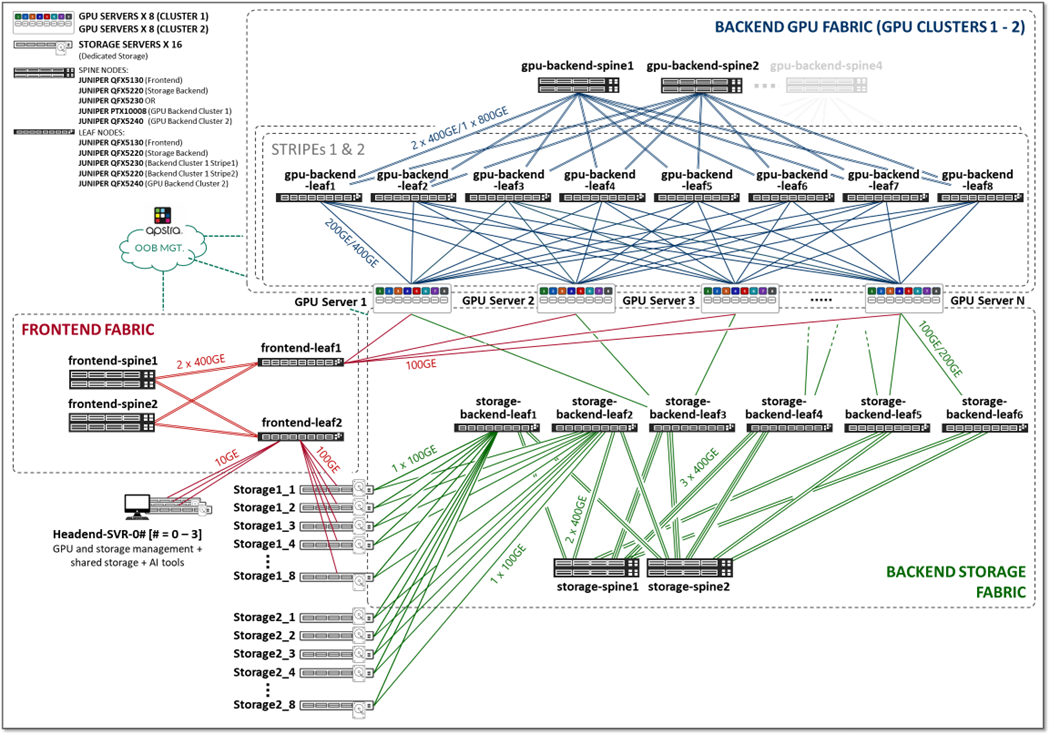
The three fabrics described in the previous section (Frontend, GPU Backend, and Storage Backend), are interconnected together in the overall AI JVD solution architecture as shown in Figure 2.

Figure 2: AI JVD Solution Architecture

We have built two different Clusters, as shown in Figure 3, which share the Frontend fabric and Storage Backend fabric but have separate GPU Backend fabrics . Each cluster is made of two stripes following the Rail Optimized Stripe Architecture , but include different switch models as Leaf and Spine nodes, as well as GPU server models.

Figure 3: AI JVD Lab Clusters

The GPU Backend in Cluster 1 consists of Juniper QFX5220, and QFX5230 switches as leaf nodes and either QFX5230s switches or PTX10008 routers acting as spine nodes and includes Nvidia A100 GPU servers. The QFX5230s and PTX10008 acting as spine nodes have been validated separately, while maintaining the leaf nodes the same. Apstra blueprints are used to switch between the setups with QFX5230s acting as spine nodes and the one with PTX10008 acting as spine.

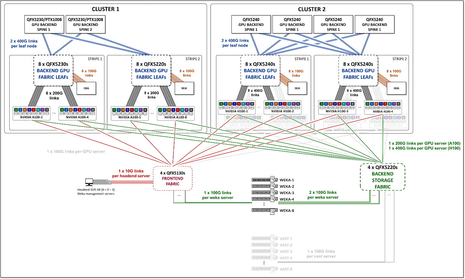
The GPU Backend in Cluster 2 consists of Juniper QFX5240 switches acting as both leaf nodes and spine nodes and includes AMD MI300X GPU servers and Nvidia H100 GPU servers.

The rest of this document focuses on the Nvidia servers and Weka storage and includes server and storage configurations, specific for these systems.

It is important to notice that the type of switch and the number of switches acting as leaf and spine nodes, as well as the number and speed of the links between them, is determined by the type of fabric (Frontend, GPU Backend or Storage Backend) as they present different requirements. More details will be included in the respective fabric description sections.

In the case of the GPU Backend fabric, the number of GPU servers, as well as the number of GPUs per server, are also factors determining the number and switch type of the leaf and spine nodes.