Probes Introduction
Probes are the basic unit of abstraction in Intent-Based Analytics. Generally, a given probe consumes some set of data from the network, does various successive aggregations and calculations on it, and optionally specifies some conditions of said aggregations and calculations on which anomalies are raised.
Probes are Directed Acyclic Graphs (DAGs) where the nodes of the graph are processors and stages. Stages are data, associated with context, that can be inspected by the operator. Processors are sets of operations that produce and reduce output data from input data. The input to processors are one-or-many stages, and the output from processors are also one-or-many stages. The directionality of the edges in a probe DAG represent this input-to-output flow.
Importantly, the initial processors in a probe are special and do not have any input stage. They are notionally generators of data. We shall refer to these as source processors.
IBA works by ingesting raw telemetry from collectors into probes to extract knowledge (ex: anomalies, aggregations and so on). A given collector publishes telemetry as a collection of metrics, where each metric has identity (viz, set of key-value pairs) and a value. IBA probes, often with the use of graph queries, must fully specify the identity of a metric to ingest its value into the probe. With this feature, probes can ingest metrics with partial specification of identity using ingestion filters, thus enabling ingestion of metrics with unknown identities.
Some probes are created automatically. These probes will not be deleted automatically. This keeps things simple operationally and implementation-wise.
Processors
The input processors of a probe handle the required configuration to ingest raw telemetry
into the probe to kickstart the data processing pipeline. For these processors, the number
of stage output items (one or many) is equal to the number of results in the specified graph
query(s). If multiple graph queries are specified, for example. graph_query: [A,
B], and query A matches 5 nodes and query B matches 10 nodes, results of query A
will be accessible using query_result indices from 0 to 4, and results of
query B using indices from 5 to 14.
If a processor's input type and/or output type is not specified, then the processor takes a single input called in, and produces a single output called out.
Some processor fields are called expressions. In some cases, they are graph
queries and are so noted. In other cases, they are Python expressions that
yield a value. For example, in the Accumulate processor, duration may be specified as
integer with seconds, for example 900, or as an expression, for example
60 * 15. However, expressions could be more useful: there are multiple
ways to parameterize them.
Expressions support string values. Processor configuration parameters that are strings and
support expressions should use special quoting when specifying static value. For example,
state: "up" is not valid because it refers to the variable "up", not a
static string, so it should be: state: '"up"'.
An expression is always associated with a graph query and is run for every resulting match of that query. The execution context of the expression is such that every variable specified in the query resolves to a named node in the associated match result. For more information, see Service Data Collector example.
Graph-based processors have been extended with query_tag_filter, which enables you to filter graph query results by tags. In IBA probes, tags are used only as filter criteria for servers and external routers, specifically for the ECMP Imbalance (External Interfaces) probe and the Total East/West Traffic probe. For specific processor information, see Probe Processors in the References section.
Ingestion Filters
With "ingestion filters" one query result can ingest multiple metrics into a probe. Table
data types are used to store multiple metrics as part of a single stage output item. Table
data types include table_ns, table_dss,
table_ts - to correspond to existing types - ns,
dss, ts -respectively.
IBA Collection Filter
Collection filters determine the metrics that are collected from the target devices.
A collection filter for a given collector on a given device, is simply a collection of ingestion filters present in different probes. You can also specify it as part of enabling a service outside the context of IBA or probes but existing precedence rules for service enablement apply here - only filters at a given precedence level are aggregated. When multiple probes specify an ingestion filter targeting a specific service on a specific device, the metrics collected are a union - in other words, a metric is published when it matches any of the filters. This is why, the data is also filtered by the controller component prior to ingesting into the IBA probes.
This filter is evaluated by telemetry collectors, often to better control even what subset of available metrics is fetched from the underlying device operating system (for example, to fetch only a subset of routes instead of getting all routes, which can be a huge number). In any case, only the metrics matching the collection filter are published as the raw telemetry.
As part of enabling a service on a device, you can now specify collection filters for services. This filter becomes an additional input provided to collectors as part of "self.service_config.collection_filters".
IBA Filter Format
Following are the design/usability goals for filters (ingestion and collection)
- Ease of authoring - given probe authors are the ones specifying it
- Most often cases are match any, match against a given list of possible values, equality match, range check if key has numeric values.
- Efficient evaluation - given the filters are evaluated in the hot paths of collection or ingestion.
- Aggregatable - multiple filters are aggregated so this aggregation logic need not become the responsibility of individual collectors.
- Programming language neutral - components operating on filters can be in Python or C++ or some other language in future.
- Programmable - be amenable to future programmability around the filters, by the controller itself and/or collectors, to enhance things like usability, performance and so on.
Considering the above goals, following is a suggested and illustrative schema for filter1. Refer to ingestion filter sections for specific examples to understand this better.
FILTER_SCHEMA = s.Dict(s.Object(
  'type': s.Enum(['any', 'equals', 'list', 'pattern', 'range', 'prefix']),
  'value': s.OneOf({
    'equals': s.OneOf([s.String(), s.Integer()]),
    'list': s.List(s.String(), validate=s.Length(min=1)),
    'pattern': s.List(s.String(), validate=s.Length(min=1)),
    'range': s.AnomalyRange(), validate=s.Length(min=1),
    'prefix': s.Object({
      'prefixsubnet': s.Ipv6orIpv4NetworkAddress(),
      'ge_mask': s.Optional(s.Integer()),
      'le_mask': s.Optional(s.Integer()),
      'eq_mask': s.Optional(s.Integer())
  })
), key_type=s.String(description=
  'Name of the key in metric identity. Missing metric identity keys are '
  'assumed to match any value'))
One instance of filter specification is interpreted as AND of all specified keys (aka per-key constraints). Multiple filter specifications coming from multiple probes are considered as OR at the filter level.
The schema presented here is only for communicating the requirements. You can choose any way that accomplishes stated use cases.
Collector Processors additional_properties specified in collector processors' configuration
can be accessed using the special context. namespace. For example, if a
collector defines property system_role, it could be used this way:
duration: 60 * (15 if context.system_role == "leaf" else 10)
Items context is available as long as the items set is unchanged from the original set derived from the collector processor configuration. After data goes through a processor that changes this set, it's no longer available (for example, any grouping processor).
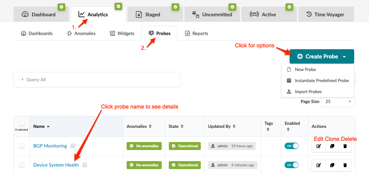
From the blueprint, navigate to Analytics > Probes to go to the probes table view. To go to a probe's details, click its name. You can instantiate, create, clone, edit, delete, import, and export probes. The screenshot below is for Apstra version 4.2.0. In Apstra version 4.2.1, some menu tabs have been renamed, moved, and/or added.
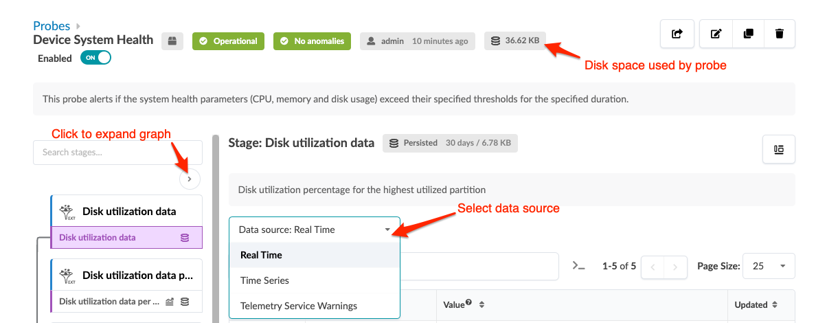
You can display stages in some probes in various ways. For example, when you click the probe named Device System Health, you'll see the image below. You can change the data source from Real Time to Time Series, then aggregate data in various ways. Also, you can see the disk space used on each probe, as applicable.
If the Apstra controller has insufficient disk space, older telemetry data files are deleted. To retain older telemetry data, you can increase capacity with Apstra VM Clusters.
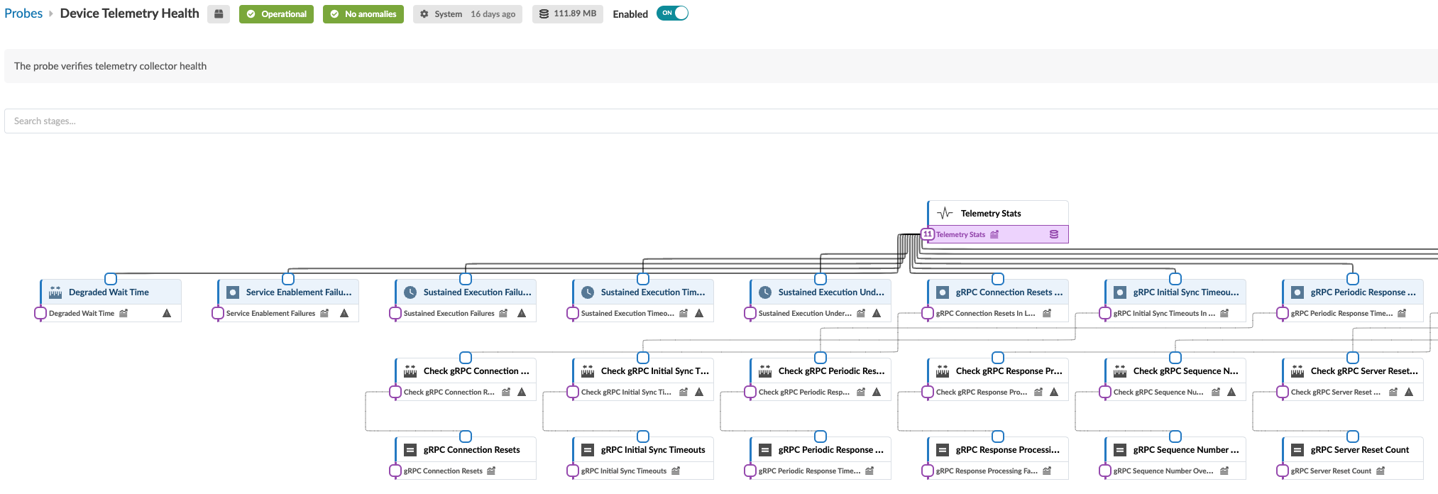
The structure and logic of non-linear probes with tens of processors is not easily distinguished in the standard view. You can click the expand button (top of left panel) to see an expanded representation of how the processors are inter-related. For example, the image below shows part of the expanded view of the Device Telemetry Health probe.
Data Sources
On applicable stages, you can specify the source to use for collecting data, either real time or time series. With time series, you can customize the manner in which the data is collected as follows:
-
Aggregation type (new in Apstra version 4.2.0)
-
None
-
allOf - boolean - True if true for all samples in the period
-
anyOf - boolean - True if true for at least one of the samples in the period
-
Average - average value in the aggregation period
-
Last - last value in the aggregation period
-
Max - maximum value in the aggregation period
-
Min - minimum value in the aggregation period
-
-
Aggregation Period (Off or a specfied number of seconds, minutes, hours or days)
-
How far back in time to collect (the last number of minutes, hours, or days)